6 Sampling assumptions
So far, we’ve seen where strong sampling was a logical assumption to make. But it isn’t always.
For example, consider the hormone problem from Chapter 3. If you were randomly testing people’s hormone levels and every person just happened to be healthy, clearly strong sampling wouldn’t be appropriate, because we were sampling from the full population of both healthy and unhealthy people.
This raises a question: Are people sensitive to the process by which data are generated?
Spoiler alert: Yes.
6.1 Word learning 💬
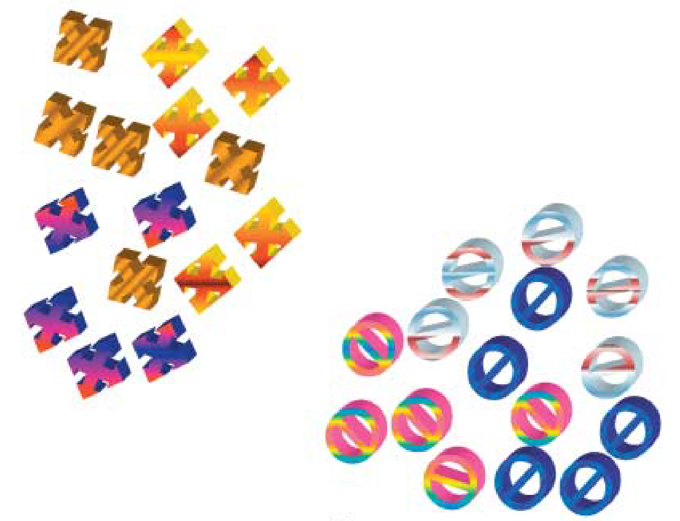
Suppose you see the following collection of objects on a table.

Now consider the following situation:
A teacher picks three blue circles from the pile and calls them “wugs”.
What is a wug? Are all circles wugs? Or just blue circles?
Consider a different situation:
A teacher picks one blue circle from the pile and calls it a “wug”. The teacher then asks a child to choose two more (the child picks two blue circles). The teacher confirms that they are also wugs.
What is a wug? Are all circles wugs? Or just blue circles?
In both situations, the observed data is the same: three blue circles labeled as wugs. What’s different is the process by which the data were generated. In one case, a knowledgeable teacher picked all the wugs; in the other, the teacher only picked one example and a (probably not knowledgeable) child picked the others.
To use some terms we’ve seen before, the teacher is using strong sampling. The child is using something closer to weak sampling.

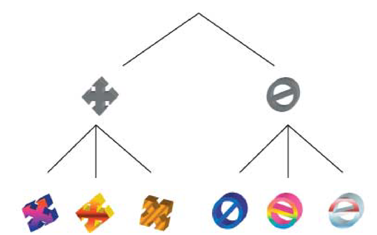
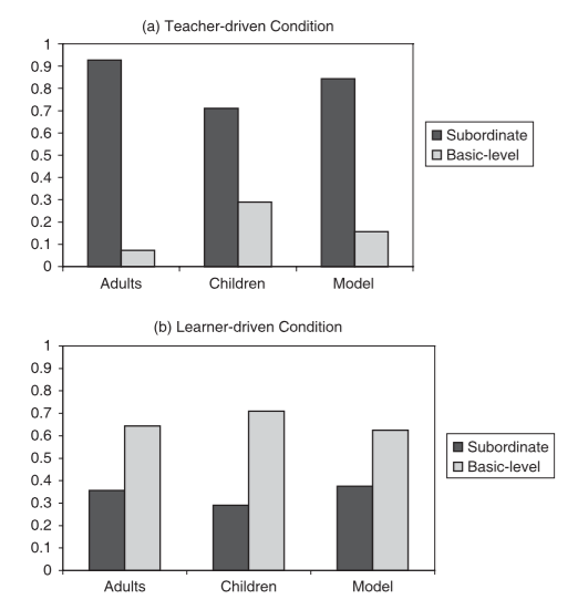
This is based on an actual study by Fei Xu and Josh Tenenbaum, who also developed a model of the task. They asked whether children and adults would generalize the word “wug” to the basic-level category (circles with lines in them) or the subordinate category (blue circles with lines in them). Here are their results:

People clearly distinguished between the teacher-driven situation and the child-driven (learner-driven) situation, and were much more likely to generalize “wugs” to the subordinate category when the teacher picked the objects.
6.2 Pedagogical sampling 🧑🏫
The teacher choosing wugs could be said to be using pedagogical sampling. The teacher deliberately used knowledge of the wug concept to select informative examples to help the child learn the concept as quickly as possible.
This is an idea explored by Patrick Shafto, Noah Goodman, and Thomas Griffiths (as well as Elizabeth Bonawitz and other researchers in related work). To put it in formal terms:
\[ \begin{equation} P_{\text{teacher}}(d|h) \propto (P_{\text{learner}}(h|d))^\alpha \end{equation} \tag{6.1}\]
Here, \(\alpha\) is a parameter that controls how optimized the teacher’s choices are. As \(\alpha \rightarrow \infty\), the teacher will choose examples \(d\) that maximize the learner’s posterior probability.
We can figure out how the learner will update their beliefs about a concept by directly applying Bayes rule:
\[ \begin{equation} P_{\text{learner}}(h|d) = \frac{P_{\text{teacher}}(d|h)P(h)}{\sum_{h_i} P_{\text{teacher}}(d|h_i)P(h_i)} \end{equation} \tag{6.2}\]
This equation makes it clear that the teacher and learner are inextricably linked: The teacher chooses examples to maximize the learner’s understanding, and the learner updates beliefs based on expectations of how the teacher is choosing examples. The model is recursive.
As the researchers explain in their paper, the two equations above are a system of equations that can be rearranged to create the following equation defining how the teacher should choose examples:
\[ \begin{equation} P_{\text{teacher}}(d|h) \propto \left( \frac{P_{\text{teacher}}(d|h) P(h)}{\sum_{h_i} P_{\text{teacher}}(d|h_i) P(h_i)} \right)^\alpha \end{equation} \tag{6.3}\]
How to solve this equation? In the paper, they use an iterative algorithm, that works like this:
- Initialize \(P_{\text{teacher}}(d|h)\) using weak sampling.
- Iterate through the following steps until \(P_{\text{teacher}}(d|h)\) stabilizes (doesn’t change from one iteration to the next):
- For each possible \(h\) and \(d\), compute \(P_{\text{learner}}(h|d)\) using Equation 6.2 and \(P_{\text{teacher}}(d|h)\) values from the previous iteration.
- For each possible \(d\) and \(h\), update \(P_{\text{teacher}}(d|h)\) using \(P_{\text{learner}}(h|d)\) values from the previous step, where \(P_{\text{teacher}}(d|h_i) = P_{\text{learner}}(h_i|d) / \sum_{d_j} P_{\text{learner}}(h_i|d_j)\) (Equation 6.1).
6.2.1 The rectangle game
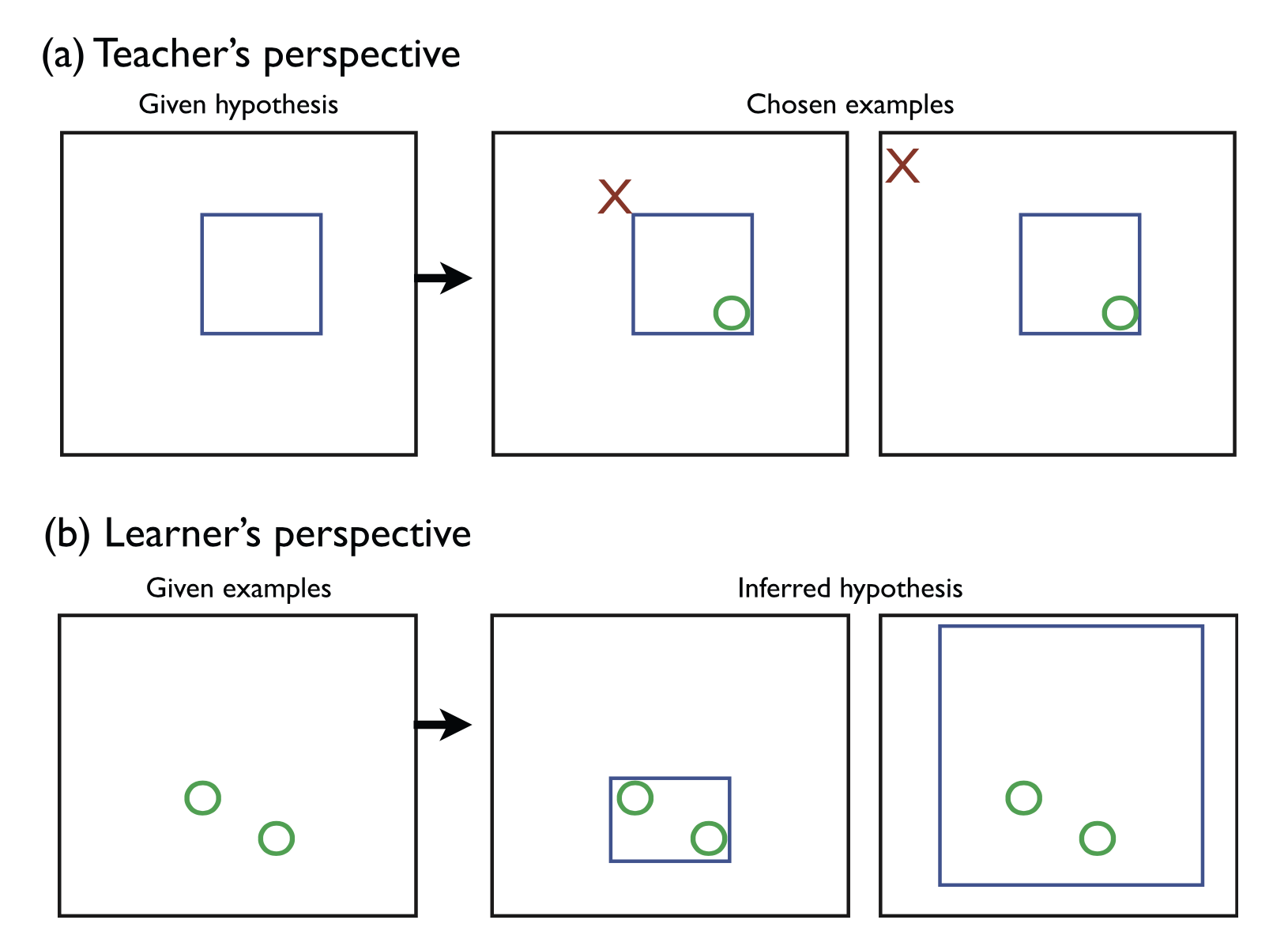
The researchers tested out their model in an experiment using a simple task called the rectangle game.
In the game, concepts are rectangular boundaries in a two-dimensional space. The teacher knows the boundary and the learner has to figure it out from examples given by the teacher.

In one version, the teacher can only provide positive examples (“Here’s an example that’s inside the boundary”). In another version, the teacher can also provide negative examples (“Here’s an example that’s not inside the boundary”).
In an experiment, they asked people to play the role of the learner in the rectangle game. There were three conditions:
- Teaching-pedagogical learning: People first acted as teachers, then as learners.
- Pedagogical learning: People acted just as learners and were told the examples they saw were chosen by a teacher.
- Non-pedagogical learning: People acted just as learners and were told the examples they saw were not chosen by a teacher.
After showing people examples, they asked them to draw a rectangle of their best guess about what the boundary was.
One key prediction of the model is that the most informative locations for examples under pedagogical sampling are at the corners of the rectangles. To test whether the learners understood this, they measured the proportion of examples that ended up in the corners of the rectangles people drew. The results are shown below.

As you can see, when people thought a knowledgeable teacher was providing the examples (the teaching-pedagogical and pedagogical learning conditions), they were much more likely to draw tight boundaries around the examples, compared to when they didn’t think a teacher was providing the examples (the non-pedagogical learning condition). This suggests that people were indeed sensitive to the process by which the data were generated and incorporated that understanding into their inferences.
6.2.2 Why the hypothesis space matters
What happens when teachers and learners have different assumptions about the the problem they’re looking at?
In the rectangle game, it’s pretty obvious what the space of hypotheses is: it’s practically pre-specified as part of the game. But in most real-world teaching situations, teachers have much more knowledge not shared by the learners than just the specific concept they are trying to convey. How might this interfere with learning?
This was the question that a group of researchers led by Rosie Aboody tested. They applied the model we just looked at to a problem where the space of hypotheses was more ambiguous than in the rectangle game. In a study of 220 people (20 teachers and 200 learners), only about half of the learners managed to fully learn the concept (a rule in this case). They used the model to better understand what was going on.
They input the teachers’ chosen examples into the model to see if the model successfully learned the correct rule. What they varied was the hypothesis space of possible rules the model considered. When the hypothesis space was small (55 or fewer total rules), the model inferred the correct rule for 75% of the teachers’ sets of examples (by correct, they mean placing 95% or more posterior probability on the correct rule). It wasn’t until they increased the hypothesis space to 95 total rules that the percentage of times the teachers’ examples led the model to correctly infer the rule dropped to 55%.
The researchers concluded from this that the learners were probably considering a larger, more complex set of rules than the teachers were. This misaligned set of assumptions likely caused the low learning rate.
In the next chapter, we’ll work through one more application of people’s sensitivity to different sampling assumptions: understanding the pragmatics of speech.